Beyond Isotropy in JEPAs: Hamiltonian Geometry and Symplectic Prediction

by Robert Jenkinson Álvarez

Accepted to NeurIPS 2026 Main Track–Poster

JEPAs usually target an isotropic latent cloud; HamJEPA instead predicts between views with a symplectic map on phase space.

Geometric ML

  • ImageNet-100 q linear probe: 31.92 vs 24.40
  • q kNN: 24.92 vs 20.10 at 45 epochs

Downloadable summary PDF: open PDF.

1. The main theoretical move

A common JEPA instinct is to regularize toward an isotropic Gaussian because isotropy appears generic. Isotropic regularization already imposes the ambient Euclidean metric as the symmetry reference. If downstream tasks have structure, that reference frame can be wrong.

The formal setup introduces a structured SPD operator \(H\succ0\), downstream task family

\[ y=w^\top \tilde{z}, \qquad \mathcal W_H=\{w:w^\top H^{-1}w\le 1\}, \]

and an \(H\)-energy budget

\[ \operatorname{tr}(H\Sigma)=c, \qquad \Sigma=\operatorname{Cov}(\tilde{z}). \]

Under this geometry, the unique minimax covariance is

\[ \Sigma^\star=\frac{c}{d}H^{-1}, \]

and the unique maximum-entropy law under the same budget is

\[ \tilde{z}\sim \mathcal{N}\!\left(0,\frac{c}{d}H^{-1}\right). \]

So the canonical object is anisotropic in ambient coordinates and isotropic only after whitening by \(H^{1/2}\).

HamJEPA pipeline: image, augmentations, shared encoder, phase-space states, symplectic predictor, and losses Diagram copied from the old working Astro site. image x τa τb view va view vb shared encoder Eθ sa qa pa sb qb pb symplectic flow ΦφK ŝb q̂b p̂b prediction loss encoder-side anti-collapse regularizers
HamJEPA at the highest level. Two augmented views of the same image are encoded by a shared encoder into phase-space states sa=[qa;pa] and sb=[qb;pb]. The predictor is not an unconstrained regression head: it is a structured Hamiltonian rollout ΦφK that evolves sa into a predicted target state ŝb. Training combines a prediction loss between ŝb and sb with separate encoder-side anti-collapse regularizers applied across the batch of states.

2. The price of using the wrong sphere

If Euclidean isotropy is imposed anyway, the feasible isotropic covariance under the same budget is

\[ \Sigma_{\mathrm{iso}}=\frac{c}{\operatorname{tr}(H)}I, \]

and the worst-case variance ratio becomes

\[ \rho(H)=\frac{V(\Sigma_{\mathrm{iso}})}{V(\Sigma^\star)} =\frac{d\,\lambda_{\max}(H)}{\operatorname{tr}(H)}, \qquad 1\le \rho(H)\le d. \]

The price of isotropy is that isotropic regularization is only metric-consistent when \(H\propto I\).

A phase-space bridge is then introduced via

\[ \mathcal H_H(q,p)=\tfrac12 q^\top Hq+\tfrac12\|p\|_2^2, \qquad \pi_H(q,p)\propto \exp\!\Bigl(-\frac{d}{c}\mathcal H_H(q,p)\Bigr), \]

whose \(q\)-marginal is \(\mathcal N(0,(c/d)H^{-1})\) and whose \(p\)-marginal is \(\mathcal N(0,(c/d)I)\).

3. What HamJEPA actually changes

Because the relevant \(H\) is unknown in practice, HamJEPA does not hard-code a structured encoder marginal. It places Hamiltonian structure in the predictor. Each view is encoded as a phase-space state \(s=(q,p)\), with \(q\) as content coordinate and \(p\) as momentum-like auxiliary state. Cross-view prediction is performed by a \(K\)-step leapfrog rollout of

\[ \mathcal H_\phi(q,p)=\tfrac12\|p\|_2^2+V_\phi(q). \]

The predictor map \(\hat s_b=\Phi_\phi^K(s_a)\) is symplectic, volume-preserving, and reversible under time-step sign reversal. The key claim is not literal physical dynamics in the encoder; it is that the view-to-view map is no longer an arbitrary geometry-destroying regressor.

4. Symplecticity is not the same thing as anti-collapse

Symplectic structure alone does not guarantee non-collapse at the encoder output. A symplectic predictor cannot locally crush phase-space volume, but the encoder could still produce a degenerate state cloud. HamJEPA therefore adds encoder-side non-collapse terms: fixed-unit energy budgets for \(q\) and \(p\), a projected log-determinant floor, and a participation-ratio floor. These controls are intentionally weaker and more geometry-aware than forcing \(\Sigma\propto I\): they preserve scale and rank without declaring all directions equivalent.

HamJEPA leapfrog predictor: Hamiltonian decomposition and kick-drift-kick rollout Diagram copied from the old working Astro site. sa q p Hφ(q,p)=T(p)+Vφ(q) q̇ = p, ṗ = -∇qVφ(q) T(p)=½||p||² Vφ(q) one leapfrog step half-kick drift half-kick p ← p − (Δt/2)∇V(q) q ← q + Δt p p ← p − (Δt/2)∇V(q) repeat K times ŝb q̂b p̂b
What the predictor is doing. HamJEPA does not use an arbitrary predictor za→ẑb. Instead, it rolls the state forward with a learned separable Hamiltonian Hφ(q,p)=T(p)+Vφ(q) and a leapfrog integrator. The potential Vφ(q) drives the kick updates through ∇qVφ(q), while the kinetic term T(p)=½||p||² yields the drift update q←q+Δt p. Repeating this structured step K times produces the predicted target state ŝb=ΦφK(sa).

5. What is held fixed, and why that matters

The comparisons are controlled. Across methods, the JEPA backbone, augmentations, optimizer, batch size, and training schedule are held fixed. Both datasets use a headless token regime based on ResNet stage-3 features, and the projector is identity so the \(q/p\) split is not remixed by an MLP head. The intended interpretation is geometric: the observed gains are not explained by changing the surrounding recipe.

6. How to read the q/p results

At CIFAR-100 30 epochs, \(q\) is the strongest HamJEPA readout for kNN while \((q,p)\) gives the best linear probe. The interpretation is that \(q\) carries cleaner metric-consistent neighborhood structure, while \(p\) contributes complementary linearly decodable signal. On ImageNet-100, where the stable pretraining regime uses full \((q,p)\) state, HamJEPA \(q\), \(p\), and \((q,p)\) are all strong and close; for SIGReg, concatenated \((q,p)\) remains better than either half. This indicates complementarity for SIGReg versus greater redundancy and individual informativeness for HamJEPA.

7. What the numbers imply

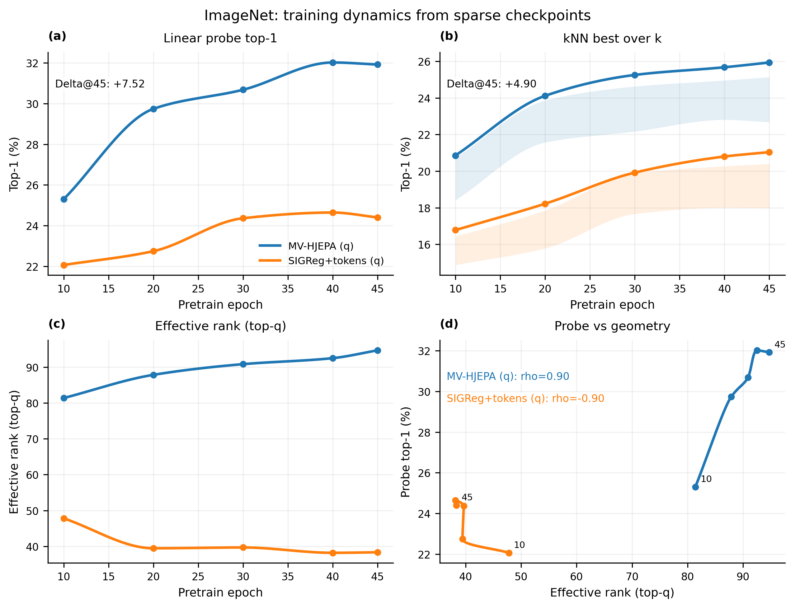
The short-budget numbers are already decisive. On CIFAR-100 at 30 epochs, HamJEPA-\(q\) moves kNN@20 from \(26.56\pm0.18\) to \(31.45\pm0.27\) and linear probe from \(30.43\pm0.30\) to \(33.95\pm0.24\), with \((q,p)\) reaching best linear probe at \(34.18\pm0.17\). On ImageNet-100 at 45 epochs, HamJEPA improves all reported readouts over SIGReg; the strict 1024-D comparison \(q\) vs \(q\) gives \(+4.82\) at kNN@20 and \(+7.52\) in linear probe. Even the 2048-D comparison is favorable: SIGReg \((q,p)\) at \(20.94 / 25.54\) versus HamJEPA \((q,p)\) at \(24.64 / 32.04\).

The geometry diagnostics support this reading. On CIFAR-100 at 30 epochs, HamJEPA-\(q\) raises the top-256 effective-rank proxy from about \(109.7\) (SIGReg) to about \(125.6\), while HamJEPA-\(p\) is more concentrated around \(79.5\). On ImageNet-100, SIGReg-\(q/p\) are around effective rank \(38\)-\(39\), whereas HamJEPA-\(q/p\) are around \(95\)-\(98\). The gains co-move with broader mean-centered covariance rather than low-rank collapse.

8. Why the 80-epoch ablation matters

The appendix ablation isolates mechanism: replacing only the symplectic leapfrog predictor with a non-symplectic residual MLP leaves linear probe much improved over SIGReg but barely lifts neighborhood quality. MLP-HJEPA peaks around \(28.30\) kNN@20, while symplectic HamJEPA reaches \(34.43\). This is direct evidence that symplectic rollout is not decorative. Phase-space parameterization plus non-isotropic spectral control explain much of linear-probe lift; the large jump in local semantic geometry is attributed to the symplectic predictor itself.

Bottom line

HamJEPA visual guide

HamJEPA has three moving parts: the encoder splits features into q,p, the predictor transports the state with a Hamiltonian rollout, and encoder-side regularizers keep the state cloud from collapsing.

1. HamJEPA full overview

Two views are encoded to phase-space states, one state is evolved by a symplectic predictor, and the predicted target is matched while encoder-side anti-collapse controls remain active.

HamJEPA pipeline: image, augmentations, shared encoder, phase-space states, symplectic predictor, and losses Diagram copied from the old working Astro site. image x τa τb view va view vb shared encoder Eθ sa qa pa sb qb pb symplectic flow ΦφK ŝb q̂b p̂b prediction loss encoder-side anti-collapse regularizers
HamJEPA at the highest level. Two augmented views of the same image are encoded by a shared encoder into phase-space states sa=[qa;pa] and sb=[qb;pb]. The predictor is not an unconstrained regression head: it is a structured Hamiltonian rollout ΦφK that evolves sa into a predicted target state ŝb. Training combines a prediction loss between ŝb and sb with separate encoder-side anti-collapse regularizers applied across the batch of states.

2. How the encoder constructs the phase-space state

The split is implemented at token level: the channel stack for each token is partitioned into q and p halves before flattening, so s=[q;p] is a construction choice with the split preserved by an identity projector.

Encoder token-split construction of the HamJEPA phase-space state Diagram copied from the old working Astro site. view v ResNet-18 token mode layer3 feature map token grid one token q half p half df channels q ∈ Rd p ∈ Rd s=[q;p] ∈ R2d identity projector preserves the q/p split
How the encoder constructs the phase-space state. HamJEPA is not just taking an arbitrary vector and renaming its halves as q and p. In the implementation, the encoder runs in token mode: an intermediate ResNet feature map is converted into a token grid, the channel stack of each token is split into a q half and a p half, and those halves are flattened across the spatial grid to form q∈Rd and p∈Rd. These are then concatenated into s=[q;p]∈R2d. This is why HamJEPA uses an identity projector: a learned MLP after the encoder would remix the coordinates and destroy the intended q/p semantics.

3. What the predictor is doing

The predictor uses a Hamiltonian rollout $H_\phi(q,p)=T(p)+V_\phi(q)$ with half-kick, drift, and half-kick updates repeated for K steps. The mapping is structured transport, not free-form regression.

HamJEPA leapfrog predictor: Hamiltonian decomposition and kick-drift-kick rollout Diagram copied from the old working Astro site. sa q p Hφ(q,p)=T(p)+Vφ(q) q̇ = p, ṗ = -∇qVφ(q) T(p)=½||p||² Vφ(q) one leapfrog step half-kick drift half-kick p ← p − (Δt/2)∇V(q) q ← q + Δt p p ← p − (Δt/2)∇V(q) repeat K times ŝb q̂b p̂b
What the predictor is doing. HamJEPA does not use an arbitrary predictor za→ẑb. Instead, it rolls the state forward with a learned separable Hamiltonian Hφ(q,p)=T(p)+Vφ(q) and a leapfrog integrator. The potential Vφ(q) drives the kick updates through ∇qVφ(q), while the kinetic term T(p)=½||p||² yields the drift update q←q+Δt p. Repeating this structured step K times produces the predicted target state ŝb=ΦφK(sa).

4. What symplectic means geometrically

Symplectic transport allows deformations but constrains local volume behavior, separating geometric transport from unconstrained collapse.

Generic map versus symplectic map geometry Diagram copied from the old working Astro site. generic learned map symplectic map
What “symplectic” means geometrically. A generic learned map can bend, stretch, and arbitrarily collapse local geometry. A symplectic map can still deform the state space, but it preserves total phase-space volume locally, i.e. |det DΦ|=1. This gives the predictor a structured notion of reversibility and ensures that the predictor itself is not the source of volume collapse.

5. Why the predictor alone is not enough

Symplecticity constrains the predictor, but it does not by itself prevent encoder collapse. A collapsed encoder could still map many different views to almost the same latent state, and a perfectly symplectic predictor would then only move around an already-degenerate state cloud.

Why the predictor alone is not enough Diagram copied from the old working Astro site. many different views shared encoder Eθ collapsed states symplectic predictor Φφ(K) still low-volume
Why the predictor alone is not enough. Even if the predictor is perfectly symplectic, the encoder could still map many different views to nearly the same latent state. In that situation the rollout acts on an already-collapsed representation. This is why HamJEPA needs a second component beyond the predictor: encoder-side anti-collapse regularization.

6. Encoder-side anti-collapse regularizers

The regularizers act on scale, variance, projected volume, spectrum, and batch mean.

Energy budget

under-scale target over-scale
Energy budget. The energy budget keeps the average per-dimension scale of q and p near a target range. It penalizes both under-scaled states (which risk collapse toward zero) and over-scaled states (which can destabilize dynamics), so the latent cloud stays at a controlled overall radius.

Variance floor

dead coordinate all coordinates active
Variance floor. The variance floor prevents individual coordinates from becoming nearly constant across the batch. Visually, it revives dead axes: instead of allowing the latent cloud to collapse onto a lower-dimensional direction, it forces each coordinate to retain a minimum amount of variation.

Projected log-det floor

healthy volume thin sheet line-like collapse
Projected log-det floor. The projected log-det floor prevents the batch representation from flattening into a very low-volume set. It does not require isotropy, but it does force the projected covariance to retain nontrivial volume, ruling out extreme degeneracies such as line-like or sheet-like collapse.

Participation-ratio / top-eigenvalue control

one dominant spike variance spread across modes
Participation-ratio floor and top-eigenvalue control. These penalties prevent the representation from surviving only through one huge dominant direction. The participation-ratio floor encourages variance to remain spread across multiple modes, while the top-eigenvalue ceiling prevents a single spike from taking over the spectrum.

Mean penalty

mean near zero μ large offset direction
Mean penalty. A large global mean can create a dominant offset direction that makes random-pair cosine similarities look artificially cone-like. The mean penalty discourages this by keeping the batch mean closer to zero, so the geometry is not dominated by a single global shift.

7. Why CIFAR-100 and ImageNet-100 use different matching choices

Matching/readout choices are dataset-regime dependent. These choices are explained so that q, p, and (q,p) comparisons are interpretable.

CIFAR-100

Emphasize matching mainly q: the content coordinate remains the cleanest readout while p stays more auxiliary.

ImageNet-100

Match the full [q;p] state: both coordinates are directly constrained and p becomes more informative.

CIFAR-100 and ImageNet-100 matching-choice comparison Diagram copied from the old working Astro site. CIFAR-100 q̂b p̂b qb pb match mainly q q is the main content coordinate; p is more auxiliary ImageNet-100 q̂b p̂b qb pb match full [q; p] both coordinates are directly constrained
Why CIFAR-100 and ImageNet-100 use different matching choices. On CIFAR-100 the training objective emphasizes the content coordinate q, so q is the cleanest downstream readout and p mainly supports the dynamics. On ImageNet-100 the stable regime was to match the full state [q;p], which directly constrains both coordinates and makes p much more informative.

8. Construction

The diagrams move from phase-space encoding to symplectic prediction, then to the regularizers that keep the encoder output non-degenerate.

Further results

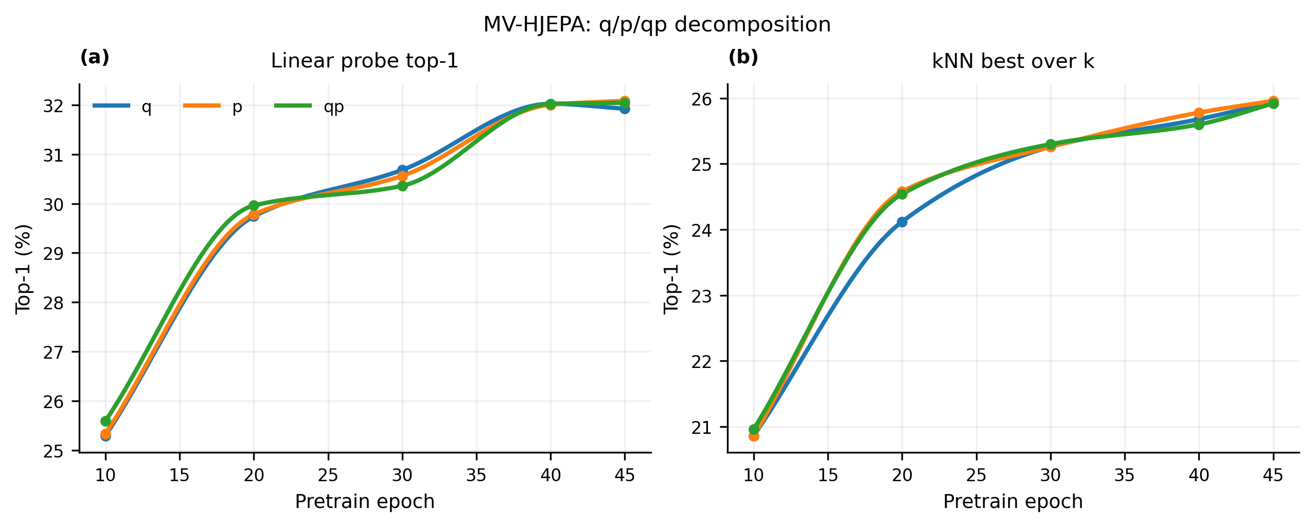
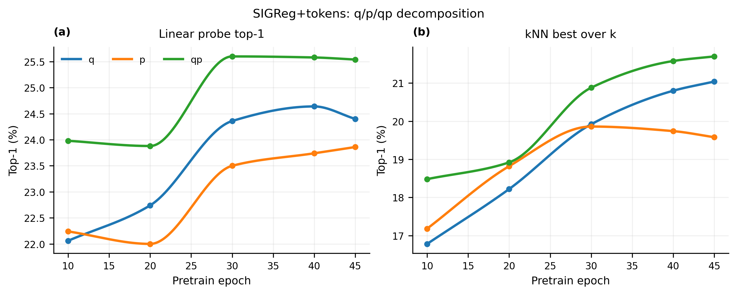
Epoch ImageNet-100 training-readout figures.

SIGReg+tokens
ImageNet-100 q/p decomposition for SIGReg tokens
q/p decomposition across pretraining (ImageNet-100). Frozen features are extracted at sparse pretraining checkpoints and evaluated with a linear probe and best kNN top-1 across evaluated k values. For SIGReg+tokens, concatenating (q,p) is consistently better than either half alone, indicating that the split halves are complementary and/or that doubling feature dimension helps.

HamJEPA

ImageNet-100 q/p decomposition for HamJEPA
For HamJEPA, q, p, and (q,p) track each other closely, suggesting that both phase-space coordinates are individually informative and largely redundant under the symplectic objective.

ImageNet-100 training dynamics

ImageNet-100 training dynamics
ImageNet-100 training dynamics from sparse checkpoints. Linear probe, best kNN, effective-rank proxy, and probe accuracy versus effective rank are shown for q. HamJEPA improves steadily and shows increasing effective rank, while SIGReg+tokens improves modestly while its effective rank decreases.

Selected geometry diagnostics

1. Videos: drift in trajectory geometry

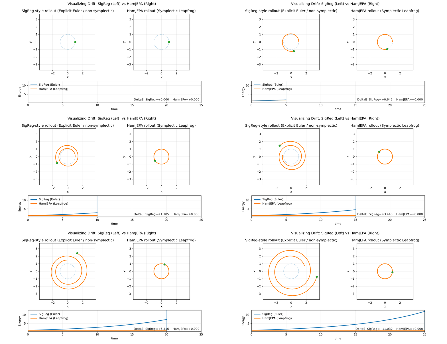
We compare rollouts by energy drift, reversibility, area preservation, symplecticity defect, and ensemble stability. Non-symplectic rollouts distort orbit structure and accumulate directional energy bias, while symplectic rollouts preserve qualitative orbit geometry with bounded oscillatory error consistent with modified-Hamiltonian intuition from backward error analysis.

Phase-plane drift
Phase-plane drift comparison
Phase-plane drift plus energy trace.

Energy surface view

Energy surface comparison for SIGReg and HamJEPA.

2. Energy drift across initial conditions

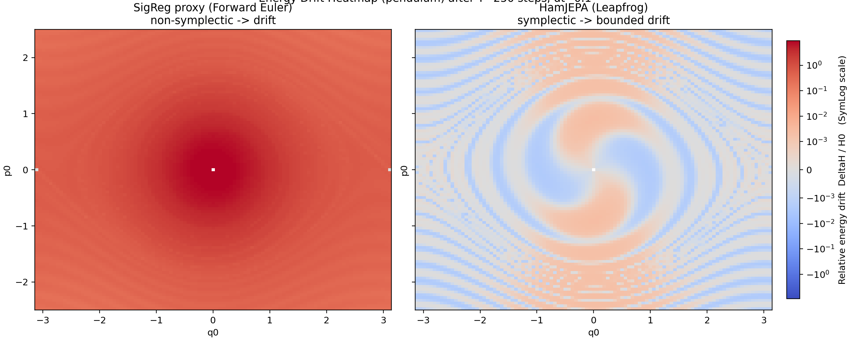
Drift is evaluated over initial states (q0, p0) using stabilized relative energy error ΔH/(H0+ε). The sym-log visualization separates near-zero residual structure from broad systematic bias; leapfrog remains balanced and bounded while Euler exhibits coherent directional accumulation.

Nonlinear pendulum drift
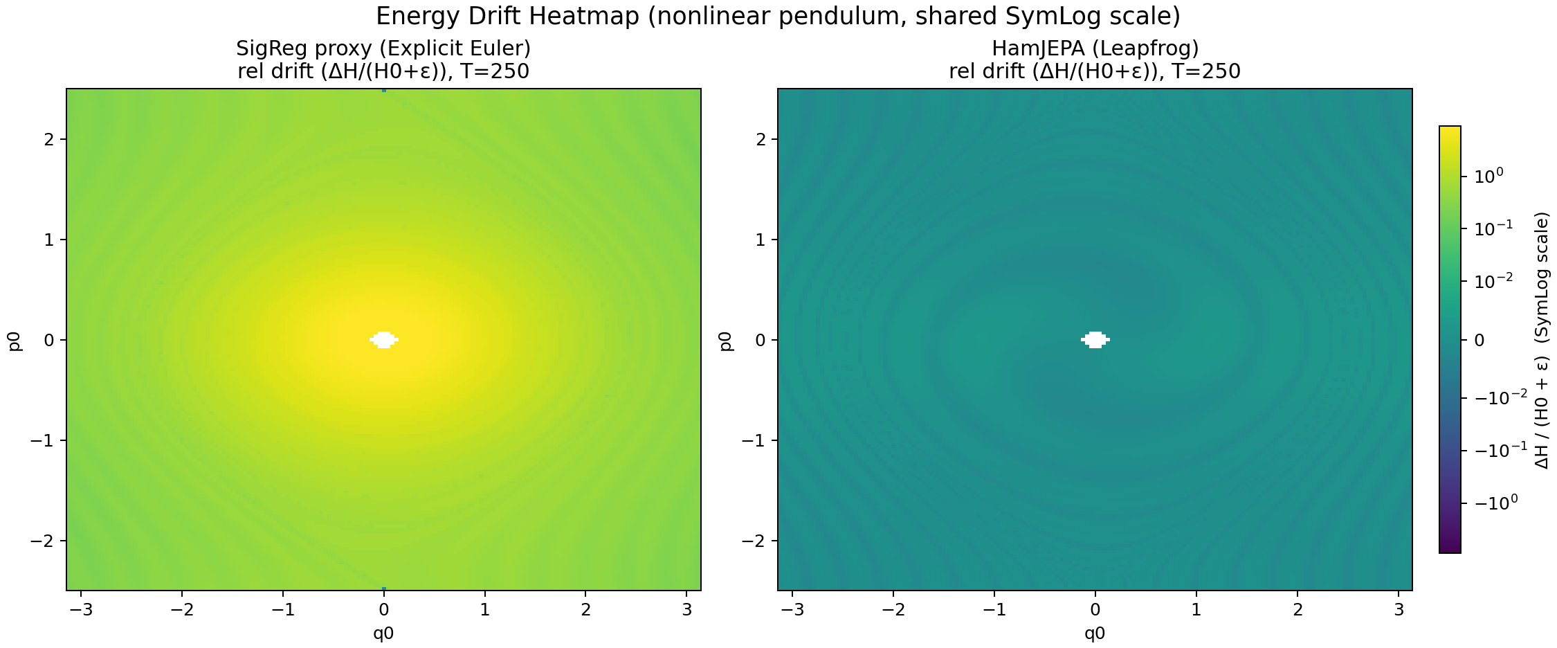
Energy drift heatmap
Drift evaluated over initial states (q0,p0).

Alternate drift view

Alternate energy drift comparison
Sym-log drift view separating near-zero residual structure from broad bias.

3. Time reversibility

Reversibility is tested by comparing a forward rollout and the reflected reverse map R(q,p)=(q,-p). Leapfrog is self-adjoint and therefore supports forward-reverse consistency; Euler is not. This diagnostic tests structural integrity, not only pointwise prediction accuracy.

Forward-reverse defect map
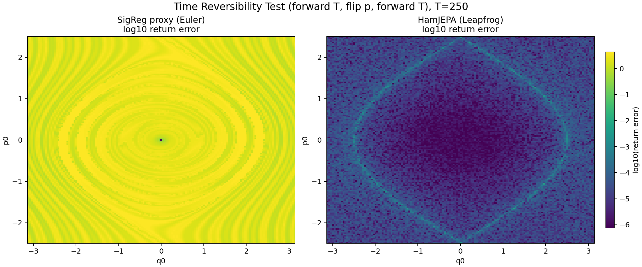
Time reversibility heatmap
Forward-reverse consistency tests structural integrity, not only point prediction.

4. Liouville / area preservation

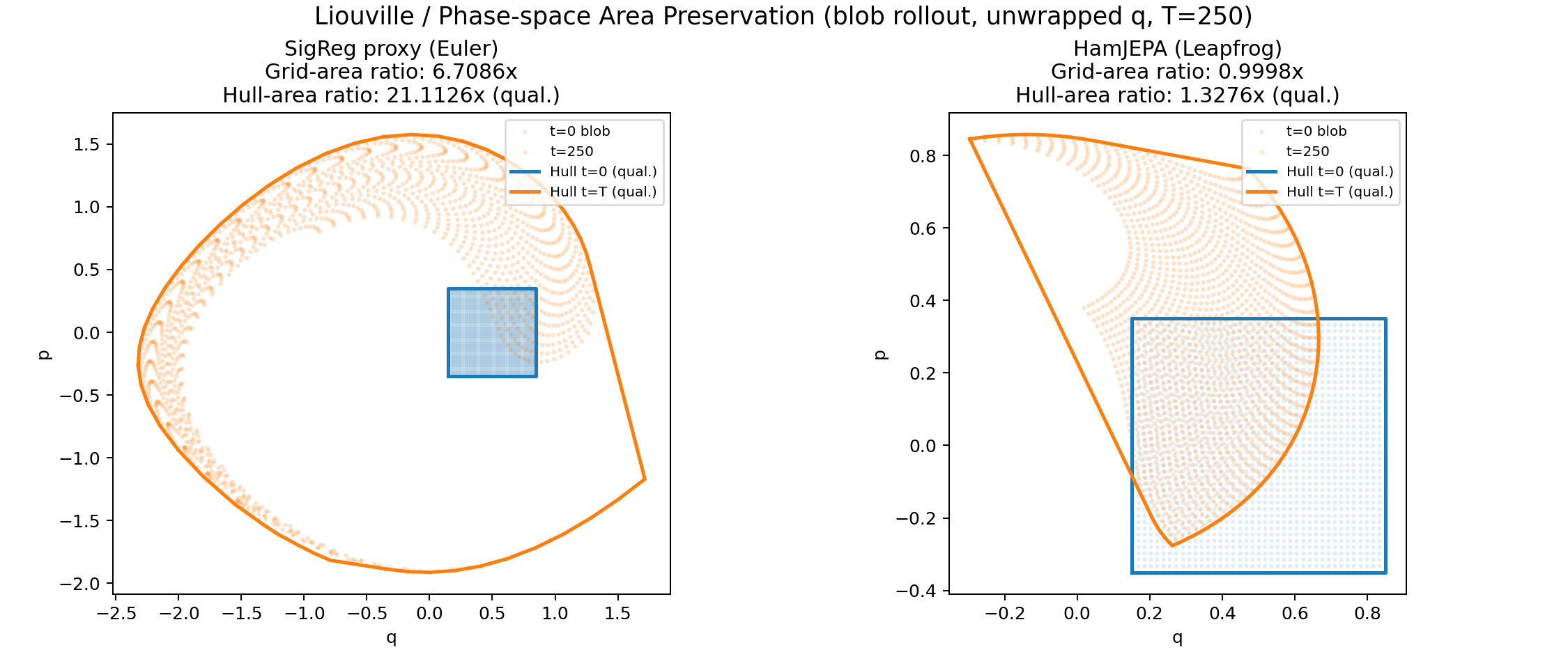
Hamiltonian flow preserves phase-space volume; in two dimensions this is area preservation. The grid-area trajectory is the quantitative diagnostic, while hull-area overlays provide qualitative deformation context. With unwrapped q, leapfrog stays near-area-preserving and Euler drifts.

Quantitative area metric
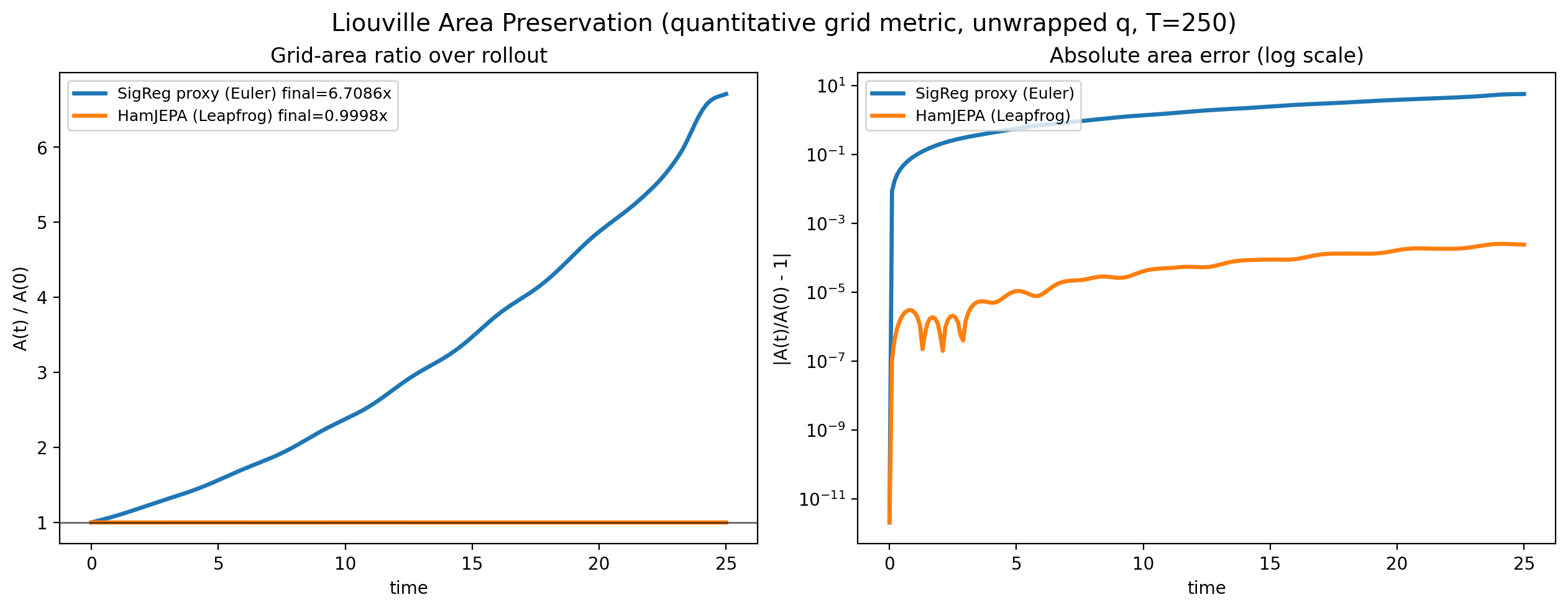
Liouville area preservation plot
Hamiltonian flow preserves phase-space volume; in two dimensions this is area preservation.

Blob deformation check

Liouville blob deformation
Hull-area overlays provide qualitative deformation context.

5. Symplecticity defect

Symplecticity is tested directly through J(x)^T Ω J(x)=Ω and defect d(x)=||J^T ΩJ-Ω||_F. This is stricter than energy drift alone and isolates structural violations; diagnostics use unwrapped coordinates and float64 Jacobians.

Defect distribution
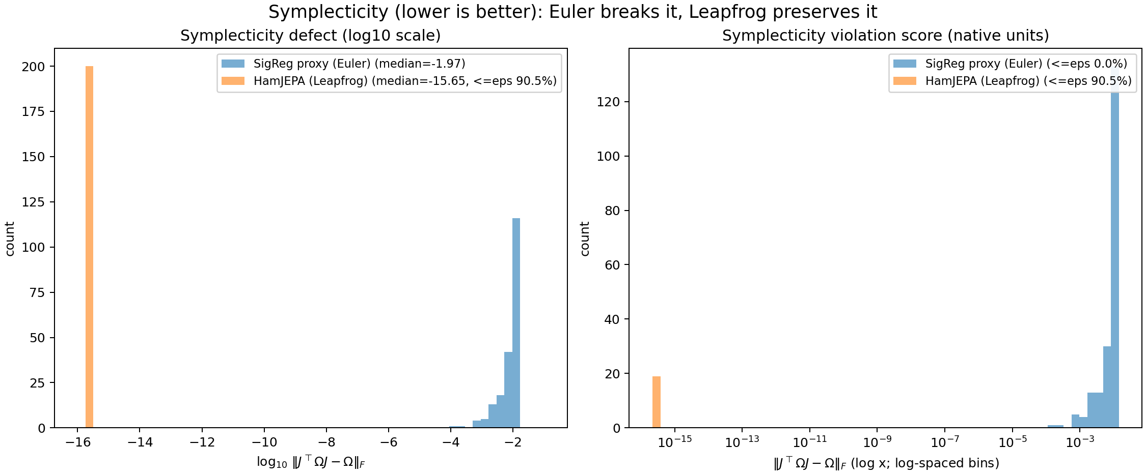
Symplecticity defect histogram
Direct test of J(x)^T Ω J(x)=Ω through Frobenius defect.

6. Long-horizon energy behavior

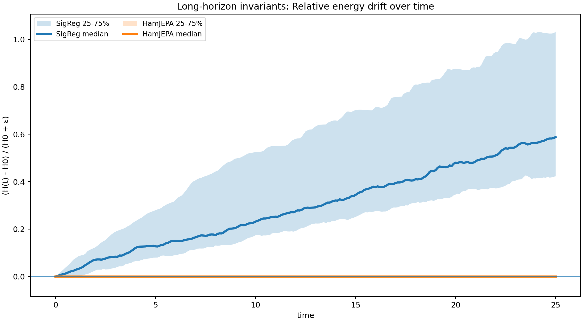
Energy error is summarized by median trajectory and IQR band, which is more robust than mean-only views under heavy-tail rollout paths. Symplectic rollout shows bounded oscillatory behavior; non-symplectic rollout shows monotone accumulation.

Median + IQR drift over time
Energy versus time
Median trajectory and IQR band summarize long-horizon energy behavior.

7. Covariance stability

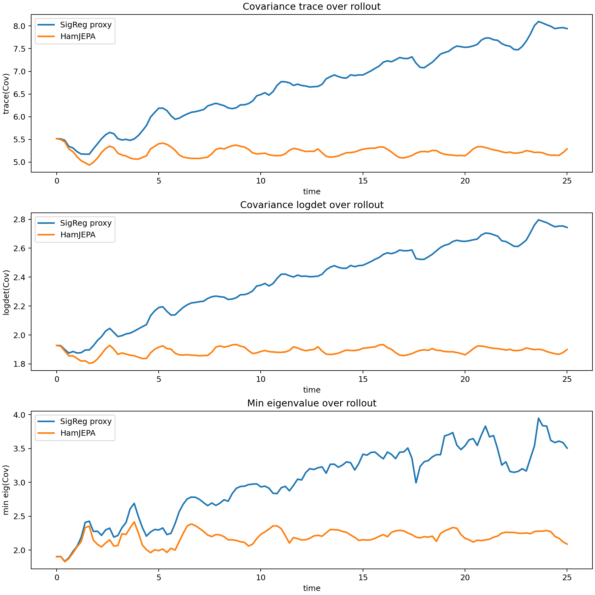
Ensemble diagnostics track tr(Cov), log det(Cov), and λ_min(Cov). These are not invariants of general nonlinear Hamiltonian flow, but they remain useful comparative indicators of rollout health and degeneration risk.

Ensemble covariance diagnostics
Covariance stability diagnostics
Ensemble diagnostics track trace, log determinant, and minimum eigenvalue of covariance.

8. Sliced-projection diagnostics

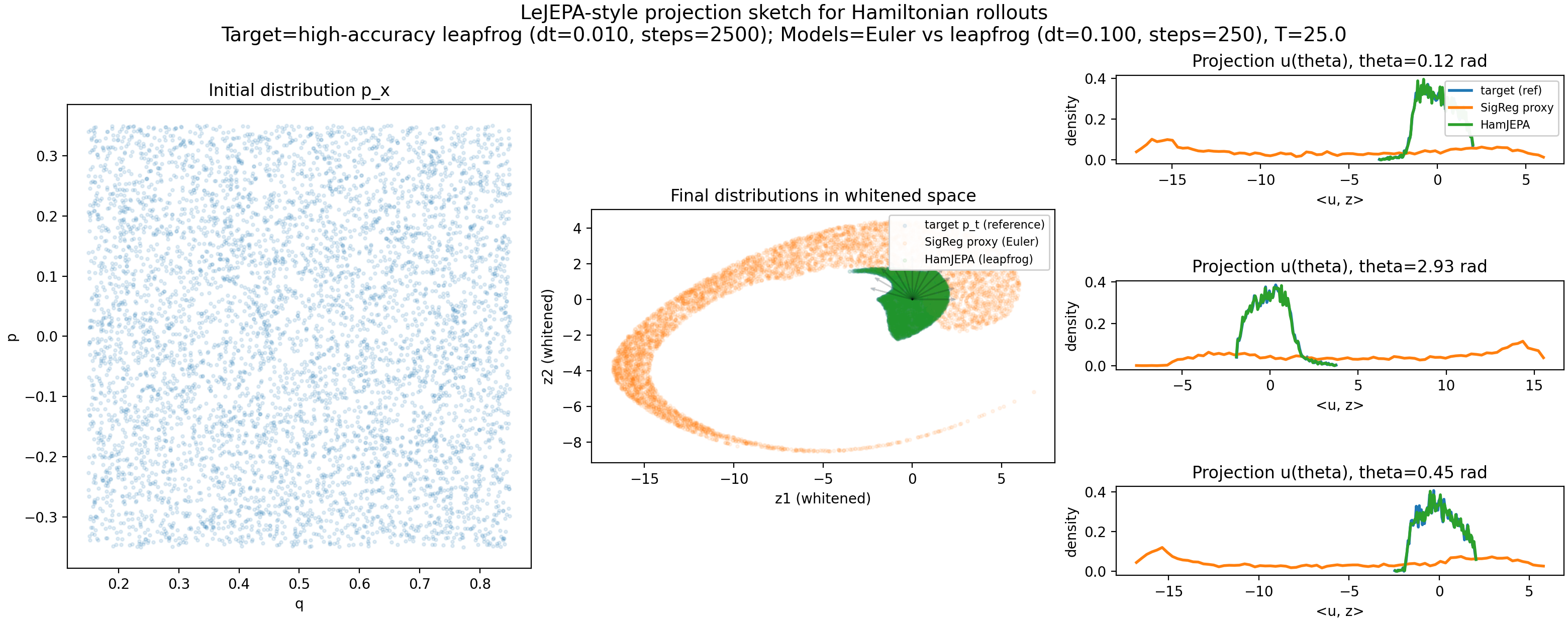
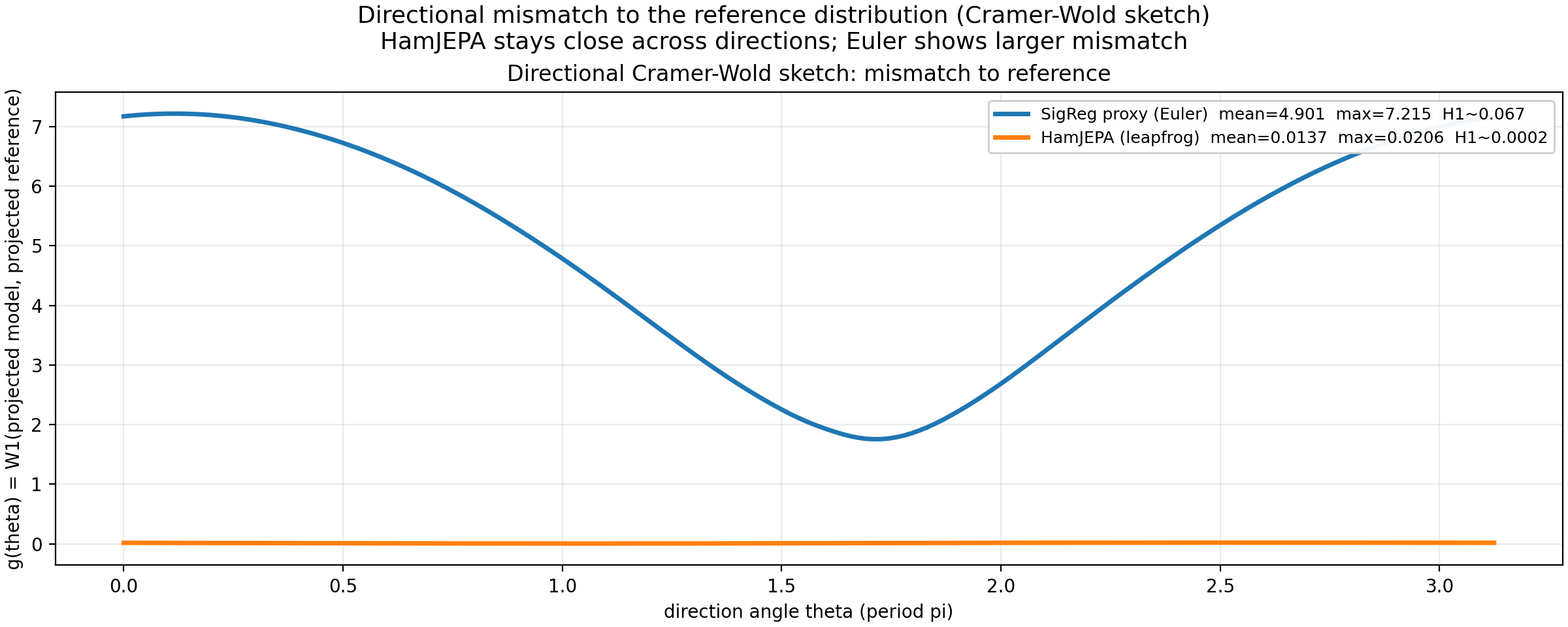
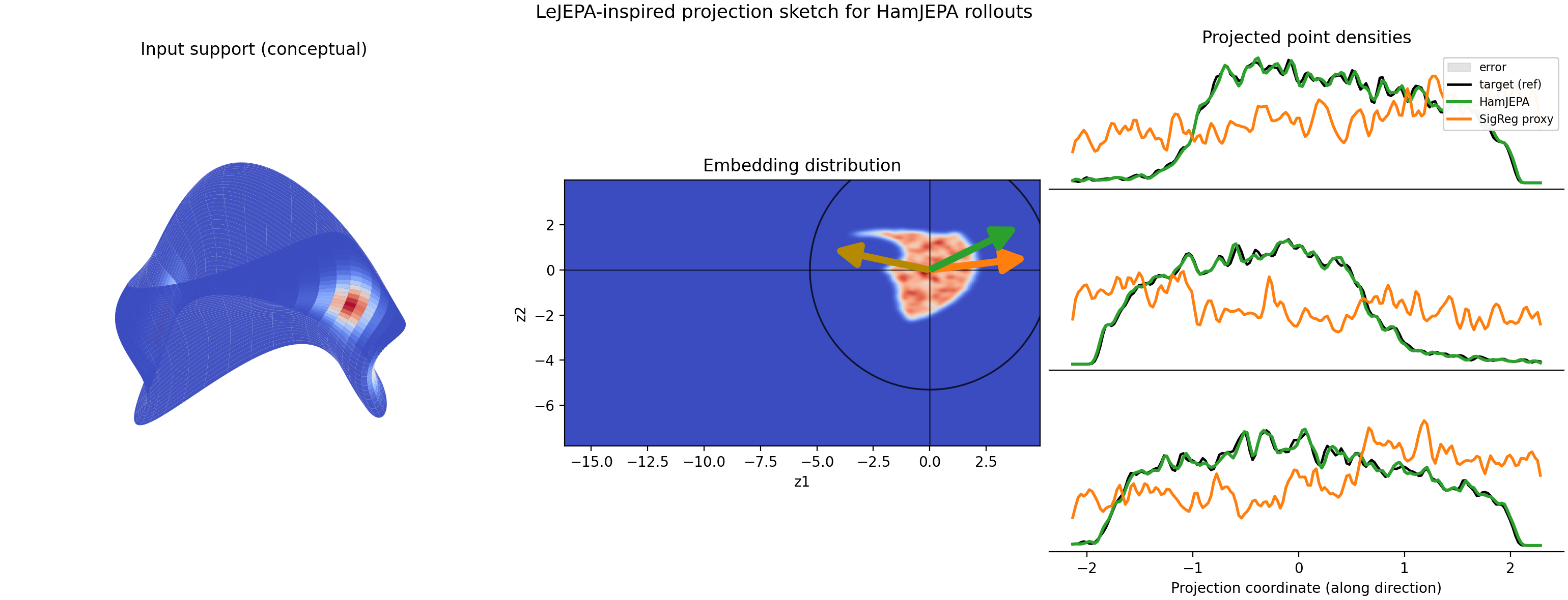
This LeJEPA paper-inspired sliced-projection diagnostic follows a Cramér-Wold viewpoint: instead of only aggregating distribution checks, compare many 1D projections to expose direction-dependent geometric distortion.

Projection cartoon
Projection cartoon
A 2D slice is projected onto many directions. Black is the reference distribution, green tracks the symplectic rollout, and orange indicates distorted non-symplectic projections.

Projection sketch

Projection sketch
Initial phase-space cloud and whitened final distributions: leapfrog remains close to the reference shape while Euler introduces directional mismatch after transport.

Directional discrepancy

Directional discrepancy curve
Direction-dependent mismatch is summarized by g(theta)=W1(<u(theta), Z_model>, <u(theta), Z_ref>). Broad peaks reveal anisotropic rollout distortion hidden by aggregate-only metrics.